《西方经济学》课程PPT教学课件（宏观经济学）Chapter 11 Application of IS-LM model

CHAPTER ELEVEN Application of IS-LM Model macroeconomics N.Gregory Mankiw College of Management,HUST

macroeconomics N. Gregory Mankiw CHAPTER ELEVEN Application of IS-LM Model macro College of Management, HUST

Learning objectives In Chapter 11,we will use the IS-LM model to see how policies and shocks affect income and the interest rate in the short run when prices are fixed derive the aggregate demand curve explore various explanations for the Great Depression CHAPTER 11 Aggregate Demand ll slide 1

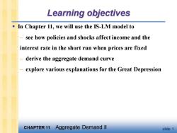
CHAPTER 11 Aggregate Demand II slide 1 Learning objectives ▪ In Chapter 11, we will use the IS-LM model to – see how policies and shocks affect income and the interest rate in the short run when prices are fixed – derive the aggregate demand curve – explore various explanations for the Great Depression

Context 1.Explaining fluctuations with IS-LM model 1.1 Policy analysis with IS-LM model 1.2 Interaction between monetary fiscal policy 1.3 Shocks in IS-LM model 2.IS-LM as a theory of aggregate demand 2.1 IS-LM model and aggregate demand 2.2 IS-LM model in short run and long run 3.The Great Depression 4,Chapter summary CHAPTER 11 Aggregate Demand ll slide 2

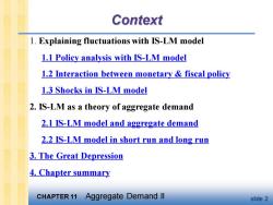
CHAPTER 11 Aggregate Demand II slide 2 Context 1. Explaining fluctuations with IS-LM model 1.1 Policy analysis with IS-LM model 1.2 Interaction between monetary & fiscal policy 1.3 Shocks in IS-LM model 2. IS-LM as a theory of aggregate demand 2.1 IS-LM model and aggregate demand 2.2 IS-LM model in short run and long run 3. The Great Depression 4. Chapter summary

1.1 Equilibrium in the /S-LM Model The IS curve represents equilibrium in the goods market. LM Y=C(Y-T)+I(r)+G The LM curve represents money market equilibrium. M/P=L(r,Y) The intersection determines the unique combination(组合)of Y and r that satisfies equilibrium in both markets. CHAPTER 11 Aggregate Demand Il slide 3

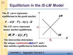
CHAPTER 11 Aggregate Demand II slide 3 The intersection determines the unique combination(组合)of Y and r that satisfies equilibrium in both markets. The LM curve represents money market equilibrium. Equilibrium in the IS-LM Model The IS curve represents equilibrium in the goods market. Y C Y T I r G = − + + ( ) ( ) M P L r Y = ( , ) IS Y r LM r1 Y1 1.1

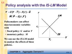
1.1 Policy analysis with the /S-LM Model Y=C(Y-T)+I(r)+G M/P=L(r,Y) LM Policymakers can affect macroeconomic variables with fiscal policy:G and/or T 。monetary policy:.M We can use the IS-LM model to analyze the effects of these policies. CHAPTER 11 Aggregate Demand ll slide 4

CHAPTER 11 Aggregate Demand II slide 4 Policy analysis with the IS-LM Model Policymakers can affect macroeconomic variables with • fiscal policy: G and/or T • monetary policy: M We can use the IS-LM model to analyze the effects of these policies. Y C Y T I r G = − + + ( ) ( ) M P L r Y = ( , ) IS Y r LM r1 Y1 1.1

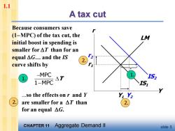
1.1 A tax cut Because consumers save (1-MPC)of the tax cut,the LM initial boost in spending is smaller for AT than for an equal△G.and the IS curve shifts by -MPC AT TS> 1-MPC I51 .so the effects on r and Y are smaller for a AT than for an equal△G. CHAPTER 11 Aggregate Demand ll slide 5

CHAPTER 11 Aggregate Demand II slide 5 IS1 1. A tax cut Y r LM r1 Y1 IS2 Y2 r2 Because consumers save (1−MPC) of the tax cut, the initial boost in spending is smaller for T than for an equal G. and the IS curve shifts by MPC 1 MPC T −  − 1. 2. 2. .so the effects on r and Y are smaller for a T than for an equal G. 2. 1.1

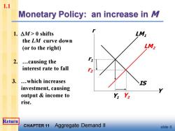
1.1 Monetary Policy:an increase in M 1.△M>0 shifts LM1 the LM curve down (or to the right) LM2 2. .causing the interest rate to fall 3. .which increases investment,causing output income to Y Y2 rise. Return CHAPTER 11 Aggregate Demand ll slide 6

CHAPTER 11 Aggregate Demand II slide 6 2. .causing the interest rate to fall IS Monetary Policy: an increase in M 1. M > 0 shifts the LM curve down (or to the right) Y r LM1 r1 Y1 Y2 r2 LM2 3. .which increases investment, causing output & income to rise. 1.1 Return

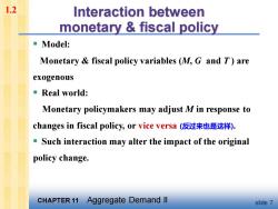
1.2 Interaction between monetary fiscal policy ■Model:: Monetary fiscal policy variables (M,G and T)are exogenous ·Real world: Monetary policymakers may adjust M in response to changes in fiscal policy,or vice versa(反过来也是这样)， Such interaction may alter the impact of the original policy change. CHAPTER 11 Aggregate Demand ll slide 7

CHAPTER 11 Aggregate Demand II slide 7 Interaction between monetary & fiscal policy ▪ Model: Monetary & fiscal policy variables (M, G and T ) are exogenous ▪ Real world: Monetary policymakers may adjust M in response to changes in fiscal policy, or vice versa (反过来也是这样). ▪ Such interaction may alter the impact of the original policy change. 1.2

1.2 The Fed's response to AG>0 Suppose Congress increases G. Possible Fed responses: 1.hold M constant 2.hold r constant 3.hold Y constant In each case,the effects of the AG are different: CHAPTER 11 Aggregate Demand ll slide 8

CHAPTER 11 Aggregate Demand II slide 8 The Fed’s response to G > 0 ▪ Suppose Congress increases G. ▪ Possible Fed responses: 1. hold M constant 2. hold r constant 3. hold Y constant ▪ In each case, the effects of the G are different: 1.2

1.2 Response 1:hold M constant If Congress raises G, the IS curve shifts right LM1 If Fed holds M constant,then LM curve doesn't shift. Results: I52 I51 △Y=Y2-Y YY2 △r=- CHAPTER 11 Aggregate Demand ll slide 9

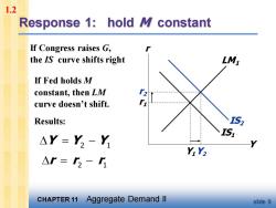
CHAPTER 11 Aggregate Demand II slide 9 If Congress raises G, the IS curve shifts right IS1 Response 1: hold M constant Y r LM1 r1 Y1 IS2 Y2 r2 If Fed holds M constant, then LM curve doesn’t shift. Results:  = − Y Y Y 2 1 2 1  = − r r r 1.2