华南师范大学：《数值计算方法》课程PPT教学课件（数值分析 Numerical Analysis）Chapter 5 Numerical Integration

善未样头导 Chapter 5 Numerical Integration

Chapter 5 Numerical Integration

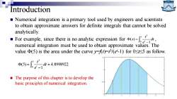
Introduction Numerical integration is a primary tool used by engineers and scientists to obtain approximate answers for definite integrals that cannot be solved analytically. For cxample.since there is no analytic exression for numerical integration must be used to obtain approximate values.The value (5)is the area under the curve )=3/(e-1)for 0t<5 as follow. 6=244s9g92 The purpose of this chapter is to develop the basic principles of numerical integration

Introduction ◼ Numerical integration is a primary tool used by engineers and scientists to obtain approximate answers for definite integrals that cannot be solved analytically. ◼ For example, since there is no analytic expression for , numerical integration must be used to obtain approximate values. The value Φ(5) is the area under the curve y=f(t)=t 3 /(e t -1) for 0≤t≤5 as follow. 3 0 ( ) 1 x t t x dt e  = −  3 5 0 (5) 4.8998922 1 t t dt e  =  −  ◼ The purpose of this chapter is to develop the basic principles of numerical integration

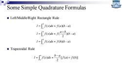
Some Simple Quadrature Formulas Left/Middle/Right Rectangle Rule 1=∫fx)dk≈fab-a) 1=∫fk*fab-a 1=fx)dk≈fbb-a) ■Trapezoidal Rule 1-few22Ua+f

Some Simple Quadrature Formulas ◼ Left/Middle/Right Rectangle Rule ◼ Trapezoidal Rule ( ) ( )( ) ( ) ( )( ) 2 ( ) ( )( ) b a b a b a I f x dx f a b a a b I f x dx f b a I f x dx f b b a =  − + =  − =  −    ( ) [ ( ) ( )] 2 b a b a I f x dx f a f b − =  + 

Left Rectangle Rule Right Rectangle Rule Middle Rectangle Rule Trapezoidal Rule

3.5 3 2.5 2 1.5 1 0.5 -0.5 -1 -1.5 -2 -2.5 -0.5 0.5 1 1.5 2 2.5 3 3.5 3.5 3 2.5 2 1.5 1 0.5 -0.5 -1 -1.5 -2 -2.5 -0.5 0.5 1 1.5 2 2.5 3 3.5 3.5 3 2.5 2 1.5 1 0.5 -0.5 -1 -1.5 -2 -2.5 -0.5 0.5 1 1.5 2 2.5 3 3.5 3.5 3 2.5 2 1.5 1 0.5 -0.5 -1 -1.5 -2 -2.5 -0.5 0.5 1 1.5 2 2.5 3 3.5 Left Rectangle Rule Middle Rectangle Rule Trapezoidal Rule Right Rectangle Rule

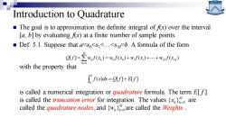
Introduction to Quadrature The goal is to approximation the definite integral offx)over the interval [a,b]by evaluatingfx)at a finite number of sample points. Def.5.1.Suppose that a=xo<x<...<xb.A formula of the form Qf1-w/(x)-w/(x)+wf(x)++wf(x) with the property that f()d+ is called a numerical integration or quadrature formula.The term E[f] is called the truncation error for integration.The values are called the quadrature nodes,and ware called the Weights

Introduction to Quadrature ◼ The goal is to approximation the definite integral of f(x) over the interval [a, b] by evaluating f(x) at a finite number of sample points. ◼ Def. 5.1. Suppose that a=x0<x1<…<xM =b. A formula of the form with the property that is called a numerical integration or quadrature formula. The term E[ f ] is called the truncation error for integration. The values are called the quadrature nodes, and are called the Weights . 0 0 1 1 0 [ ] ( ) ( ) ( ) ( ) M k k M M k Q f w f x w f x w f x w f x = = = + + +  ( ) [ ] [ ] b a f x dx Q f E f = +  0 { }M k k x = 0 { }M wk k=

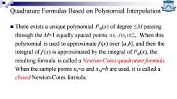
Quadrature Formulas Based on Polynomial Interpolation There exists a unique polynomial Pux)of degree <M passing through the M+1 equally spaced points {(xf()).When this polynomial is used to approximate f(x)over [a,b],and then the integral off(x)is approximated by the integral of Px),the resulting formula is called a Newton-Cotes quadrature formula When the sample points xo-a and xb are used,it is called a closed Newton-Cotes formula

Quadrature Formulas Based on Polynomial Interpolation ◼ There exists a unique polynomial PM(x) of degree ≤M passing through the M+1 equally spaced points . When this polynomial is used to approximate f (x) over [a,b], and then the integral of f (x) is approximated by the integral of PM(x), the resulting formula is called a Newton-Cotes quadrature formula. When the sample points x0 =a and xM =b are used, it is called a closed Newton-Cotes formula. 0 {( , ( ))}M k k k x f x =

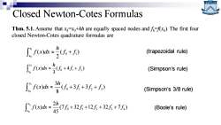
Closed Newton-Cotes Formulas Thm.5.1.Assume thatx=x+kh are equally spaced nodes andx).The first four closed Newton-Cotes quadrature formulas are fe达=96+0 (trapezoidal rule) f达*6+4f+) (Simpson's rule) e*+3++) (Simpson's 3/8 rule) 1a=治%+2+12听+2+7 (Boole's rule)

Closed Newton-Cotes Formulas 1 0 0 1 ( ) ( ) 2 x x h f x dx f f  +  2 0 0 1 2 ( ) ( 4 ) 3 x x h f x dx f f f  + +  3 0 0 1 2 3 3 ( ) ( 3 3 ) 8 x x h f x dx f f f f  + + +  Thm. 5.1. Assume that xk=x0+kh are equally spaced nodes and fk=f(xk ). The first four closed Newton-Cotes quadrature formulas are 4 0 0 1 2 3 4 2 ( ) (7 32 12 32 7 ) 45 x x h f x dx f f f f f  + + + +  (trapezoidal rule) (Simpson’s rule) (Simpson’s 3/8 rule) (Boole’s rule)

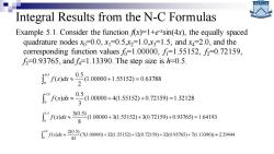
Integral Results from the N-C Formulas Example 5.1.Consider the function fx)=1+e*sin(4x),the equally spaced quadrature nodes xo-0.0,x1=0.5,x2=1.0,x3=1.5,and x4-=2.0,and the corresponding function values=1.00000,f=1.55152,=0.72159, =0.93765,and fa=1.13390.The step size is h=0.5. fa:00w0+15152=06378 [fk*051000+405152+0.72159=132128 [fd301000+315152+0.72159+093765)=164193 8 fxk÷2X0.3(71.000)+3215152+120.72159)+320.93765)+701.13390)=22944 45

Integral Results from the N-C Formulas Example 5.1. Consider the function f(x)=1+e -x sin(4x), the equally spaced quadrature nodes x0=0.0, x1=0.5,x2=1.0,x3=1.5, and x4=2.0, and the corresponding function values f0=1.00000, f1=1.55152, f2=0.72159, f3=0.93765, and f4=1.13390. The step size is h=0.5. 0.5 0 0.5 ( ) (1.00000 1.55152) 0.63788 2 f x dx  + =  1.0 0 0.5 ( ) (1.00000 4(1.55152) 0.72159) 1.32128 3 f x dx  + + =  1.5 0 3(0.5) ( ) (1.00000 3(1.55152) 3(0.72159) 0.93765) 1.64193 8 f x dx  + + + =  2.0 0 2(0.5) ( ) (7(1.00000) 32(1.55152) 12(0.72159) 32(0.93765) 7(1.13390)) 2.29444 45 f x dx  + + + + = 

The trapezoidal rule integrates Simpson's rule integrates y=P2(x) =P(x)over [xo,x1]=[0,0.5]. over [xo,x2]=[0,1]. Simpson's 3/8 rule integrates y=P3(x) Boole's rule integrates y=P4(x)over over[xo,x3]F[0,1.5]. [x0,x4]=0,2]

3.5 3 2.5 2 1.5 1 0.5 -0.5 -1 -1.5 -2 -2.5 -0.5 0.5 1 1.5 2 2.5 3 3.5 3.5 3 2.5 2 1.5 1 0.5 -0.5 -1 -1.5 -2 -2.5 -0.5 0.5 1 1.5 2 2.5 3 3.5 3.5 3 2.5 2 1.5 1 0.5 -0.5 -1 -1.5 -2 -2.5 -0.5 0.5 1 1.5 2 2.5 3 3.5 3.5 3 2.5 2 1.5 1 0.5 -0.5 -1 -1.5 -2 -2.5 -0.5 0.5 1 1.5 2 2.5 3 3.5 The trapezoidal rule integrates y=P1 (x) over [x0 , x1 ]=[0, 0.5]. Boole’s rule integrates y=P4 (x) over [x0 , x4 ]=[0, 2]. Simpson’s 3/8 rule integrates y=P3 (x) over [x0 , x3 ]=[0, 1.5]. Simpson’s rule integrates y=P2 (x) over [x0 , x2 ]=[0, 1]

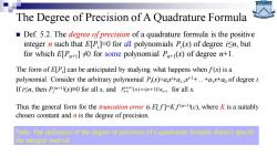
The Degree of Precision of A Quadrature Formula Def.5.2.The degree ofprecision of a quadrature formula is the positive integer n such that E[P ]0 for all polynomials P(x)of degree isn,but for which E[P]t0 for some polynomial P(x)of degree n+1. The form of E[P]can be anticipated by studying what happens when f(x)is a polynomial.Consider the arbitrary polynomial P(x)=ax+a+...+ax+ao of degree i. If isn,then P((x)=0 for allx,and P(x)=(n+1)a for all x. Thus the general form for the truncation error is E[f]=kf(D(c),where K is a suitably chosen constant and n is the degree of precision. Note:The definition of the degree of precision of a quadrature formula doesn't specify the integral interval

The Degree of Precision of A Quadrature Formula ◼ Def. 5.2. The degree of precision of a quadrature formula is the positive integer n such that E[Pi ]=0 for all polynomials Pi (x) of degree i≤n, but for which E[Pn+1] ≠0 for some polynomial Pn+1(x) of degree n+1. The form of E[Pi ] can be anticipated by studying what happens when f (x) is a polynomial. Consider the arbitrary polynomial Pi (x)=aix i+ai-1x i-1+…+a1x+a0 of degree i. If i≤n, then Pi (n+1)(x)≡0 for all x, and for all x. ( 1) 1 1 ( ) ( 1)! n P x n a n n + + + = + Thus the general form for the truncation error is E[ f ]=K f (n+1)(c), where K is a suitably chosen constant and n is the degree of precision. Note: The definition of the degree of precision of a quadrature formula doesn’t specify the integral interval