华南师范大学：《数值计算方法》课程PPT教学课件（数值分析 Numerical Analysis）Chapter 6 Solution of Differential Equations

Chapter 6 Solution of Differential Equations

Chapter 6 Solution of Differential Equations

Introduction Differential equations are commonly used for mathematical modeling in science and engineering.Often,there is no known analytic solution and numerical approximations are required. Consider the equation=1-e.It is adifferential eqution because it involves dt the derivative dy/dt of the"unknown function"yy(t). It is easy to find y(t)by integration:y(t)=t+e+C,where C is the constant of integration.By varying the value of C,we"move the solution curve"up or down, and a particular curve can be found that will pass through any desired point. The secret of the world are seldom observed as explicit formulas.Instead,we usually measure how a change in one variable affects another variable.The result is an equation involving the rate of change of the unknown function and the independent and/or denendent vorioble

Introduction ◼

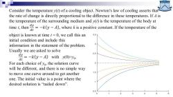
Consider the temperature y(t)of a cooling object.Newton's law of cooling asserts that the rate of change is directly proportional to the difference in these temperatures.If 4 is the temperature of the surrounding medium and y(t)is the temperature of the body at time,theny)wherei positive constant.If the temperaturefth object is known at time t=0,we call this an 3.5 initial condition and include this information in the statement of the problem. Usually we are asked to solve 2.5 =-k0y-A)with)月yo: dt For each choice of yo,the solution curve 2 will be different,and there is no simple way to move one curve around to get another 1.5 one.The initial value is a point where the desired solution is "nailed down". 0.5

Initial Value Problem Def.6.1.A solution to the initial value problem(I.V.P.) y'=ft,y)with y(to)-yo On an interval [to,b]is a differentiable function y=y(t)such that y(to)-yo and y'(t)-ft,y(t))for all tE [to,b]. Notice that the solution curve yy(t)must pass through the initial point (to,yo)

Initial Value Problem ◼

Geometric Interpretation At each point (t,y)in the rectangular region R=(t,y):a<t<b,c<td),the slope of a solution curve y=v(t)can be found using the implicit formula m-ft,y()).Hence the values m)can be computed throughout the rectangle,and each value m represents the slope of the line tangent to a solution curve that passes through the point (ti y). A slope field or direction field is a graph that indicates the slope {m over the region.It can be used to visualize how a solution curve "fits"the slope constraint. To move along a solution curve,one must start at the initial point and check the slope field to determine in which direction to move.Then take a small step from to toto+h horizontally and move the appropriate vertical distance hftoo)so that the resulting displacement has the required slope.The next point on the solution curve is(). Repeat the process to continue your journey along the curve.Since a finite number of steps will be used,the method will produce an approximation to the solution

Geometric Interpretation ◼ At each point (t, y) in the rectangular region R={(t, y):a≤t≤b, c≤t≤d}, the slope of a solution curve y=y(t) can be found using the implicit formula m=f(t, y(t)). Hence the values mi,j =f(t i , yj ) can be computed throughout the rectangle, and each value mi,j represents the slope of the line tangent to a solution curve that passes through the point (t i , yj ). ◼ A slope field or direction field is a graph that indicates the slope {mi,j} over the region. It can be used to visualize how a solution curve “fits” the slope constraint. ◼ To move along a solution curve, one must start at the initial point and check the slope field to determine in which direction to move. Then take a small step from t0 to t0+h horizontally and move the appropriate vertical distance hf(t0 ,y0 ) so that the resulting displacement has the required slope. The next point on the solution curve is (t1 ,y1 ). ◼ Repeat the process to continue your journey along the curve. Since a finite number of steps will be used, the method will produce an approximation to the solution

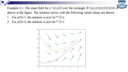
Example 6.1.The slope field for y'=(t-y)/2 over the rectangle R=(ty):05,0<4)is shown in the figure.The solution curves with the following initial values are shown: 1.For y(0)=1,the solution is v(t)=3e-42-2+t; 2.For y(0)=4,the solution is y(1)=6e42-2+t. 4.5 3.5

Example 6.1. The slope field for y’=(t-y)/2 over the rectangle R={(t,y):0≤t≤5,0≤t≤4} is shown in the figure. The solution curves with the following initial values are shown: 1. For y(0)=1, the solution is y(t)=3e -t/2 -2+t; 2. For y(0)=4, the solution is y(t)=6e -t/2 -2+t

Lipschitz condition ■Def.6.2.Given the rectangle R={(t,y):a≤b,c≤d,assume thatt,.y) is continuous on R.The function fis said to satisfy a Lipschitz condition in the variable y on R provided that a constant L>0 exists with the property that t,y)ft,y2Ll,whenever (t,y),(t,y2)ER.The constant L is called a Lipschitz constant for f. Thm.6.1.Suppose that f(t,y)is defined on the region R.If there exists a constant L>0 so that f(t,y)L for all (t,y)ER,then fsatisfies a Lipschitz condition in the variable y with Lipschitz constant L over the rectangle R

Lipschitz condition ◼

Existence and Uniqueness Thm.6.2.Assume that f(t,y)is continuous in a region R={(t,y): totb,csysd).If fsatisfies a Lipschitz condition on R in the variabley and (to,)ER,then the initial value problem in Def 6.1,y'=ft,y)with y(to)=yo,has a unique solution y=y(t)on some subinterval to<tto+. For the function ft,y)=(t-y)/2 in example 6.1,The partial derivative isf(t,y)=-1/2.Hence(t,y)1/2 and,according to Thm.6.1,the Lipschitz constant is L=1/2.Therefore,by Thm. 6.2 the I.V.P.has a unique solution

Existence and Uniqueness ◼

Euler's Method Not all initial value problems can be solved explicitly,and often it is impossible to find a formula for the solution t). For engineering and scientific purpose it is necessary to have methods for approximating the solution.If a solution with many significant digits is required,then more computing effort and a sophisticated algorithm must be used. The first approach,called Euler's method,serves to illustrate the concepts involved in the advanced methods.It has limited use because of the larger error that is accumulated as the process proceeds.However,it is important to study because the error analysis is easier to understand

Euler’s Method ◼ Not all initial value problems can be solved explicitly, and often it is impossible to find a formula for the solution y(t). ◼ For engineering and scientific purpose it is necessary to have methods for approximating the solution. If a solution with many significant digits is required, then more computing effort and a sophisticated algorithm must be used. ◼ The first approach, called Euler’s method, serves to illustrate the concepts involved in the advanced methods. It has limited use because of the larger error that is accumulated as the process proceeds. However, it is important to study because the error analysis is easier to understand

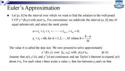
Euler's Approximation Let [a,b]be the interval over which we want to find the solution to the well-posed I.V.P.y'=ft)with y(a)=vo.For convenience we subdivide the interval [a,b]into M equal subintervals and select the mesh points a=b<h<b<.....<tv-<=b, 1=o+kh,for k=1,2....,M where h=b-a The value h is called the step size.We now proceed to solve approximately y'At,y)over [to,tul with y(to)=yo. (6.11) Assume that yt),y(t),and y(t)are continuous and use Taylor's theorem to expand y(t) about t=t.For each value t there exists a value cI that lies between to and t so that

Euler’s Approximation 0 1 2 1 0 , , for 1,2, , where . M M k a t t t t t b b a t t kh k M h M =      = − − = + = = ◼ Let [a, b] be the interval over which we want to find the solution to the well-posed I.V.P. y’=f(t,y) with y(a)=y0 . For convenience we subdivide the interval [a, b] into M equal subintervals and select the mesh points The value h is called the step size. We now proceed to solve approximately y’=f(t, y) over [t0 , tM] with y(t0 )=y0 . Assume that y(t), y’(t), and y’’(t) are continuous and use Taylor’s theorem to expand y(t) about t=t0 . For each value t there exists a value c1 that lies between t0 and t so that (6.11)