香港中文大学：《Theory of Computational Complexity》课程教学资源（讲义）Lecture 2 More samples

Lecture 2.More samples 1.Space complexity (and branching programs) 1.1 Word problem While most of the time we care time complexity,sometimes we also care space,e.g.when we do profiling of an OS kernal.Here let's see some interesting(and surprising)space-efficient algorithms. Example 3.1 Word problem.Suppose we have a string consisting four symbols,a,a,b and b1.The symbols have the property that if put adjacent,a and a cancel out,and so are b and b.So a string like abb-a is equal to the empty string.Now the question is,givena string ofn symbols,decide whether it's equal to the empty string. It's not hard to have a linear time algorithm using a stack.However,it also has linear space complexity in the worst case.(Can you design the algorithm?Can you give an instance forcing the algorithm to use linear space?) Now we consider the question of space complexity:What's the minimum space needed for any algorithm?If you think about it for some time,you may feel that there is no simple way to get an algorithm using a small amount of space,or maybe it's simply impossible.Thus the following result is quite surprising. Theorem 1.1 There is a deterministic algorithm using only O(log n)space to solve the Word problem. Consider the following two matricesand B Both matrieeshave inverse and BWe can play with these matrices by testinga few muliplications ABBA-ABAABA-00 AB=5孔BA=及引AB=E3引ABAB=8引 The first line is trivial since the matrices cancel out.The second line is interesting because that none of them happen to be identity matrix 12.This is not a coincidence---What's nice about these matrices

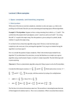
Lecture 2. More samples 1. Space complexity (and branching programs) 1.1 Word problem While most of the time we care time complexity, sometimes we also care space, e.g. when we do profiling of an OS kernal. Here let's see some interesting (and surprising) space-efficient algorithms. Example 3.1 Word problem. Suppose we have a string consisting four symbols, a, a-1 , b and b-1 . The symbols have the property that if put adjacent, a and a-1 cancel out, and so are b and b-1 . So a string like abb-1 a -1 is equal to the empty string. Now the question is, given a string of n symbols, decide whether it’s equal to the empty string. It’s not hard to have a linear time algorithm using a stack. However, it also has linear space complexity in the worst case. (Can you design the algorithm? Can you give an instance forcing the algorithm to use linear space?) Now we consider the question of space complexity: What’s the minimum space needed for any algorithm? If you think about it for some time, you may feel that there is no simple way to get an algorithm using a small amount of space, or maybe it’s simply impossible. Thus the following result is quite surprising. Theorem 1.1 There is a deterministic algorithm using only O(log n) space to solve the Word problem. Consider the following two matrices: A = [ 1 2 0 1 ] and B = [ 1 0 2 1 ]. Both matrices have inverse: A-1 = [ 1 −2 0 1 ] and B-1 = [ 1 0 −2 1 ]. We can play with these matrices by testing a few multiplications:  ABB-1A-1 = [ 1 0 0 1 ], A-1BAA-1B -1A = [ 1 0 0 1 ].  AB = [ 5 2 2 1 ], BA = [ 1 2 2 5 ], AB-1 = [ −3 2 −2 1 ], AB-1AB = [ −11 −4 −8 −3 ], … The first line is trivial since the matrices cancel out. The second line is interesting because that none of them happen to be identity matrix I2. This is not a coincidence---What’s nice about these matrices

is that,as Ivan Sanov proved in 1947,any sequence of multiplications of these matrices is not identity unless one can keep applying AA=BB1=I2 to cancel all the multiplications. Now with this,the algorithm becomes easy.Just keep multiplying the matrices and check whether finally the matrix is I2.For example,if I see abbabba'bba,thenIjust multiply ABBAB-BABBA,and at any time I only need to keep a 2x2 matrix There is one catch here:as we see from the above examples,some entries may become larger and larger as the multiplication goes on.But this turns out not to be a problem.Let's see a randomized algorithm here,and the deterministic algorithm follows from the same idea,though a few more (elementary)number theory results are needed.Pick a random prime p,and do all the computation mod p.If a matrix M is not I,then at least one entry in M-I is not 0.Then for a random prime p,the probability that the entry mod p becomes zero is very small. Remark: You've seen the essential idea ofthe algorithm.In case that you really want to make sure all details work out,here it is.Each entry can be at most exponentially large,so it only has a polynomial number of prime factors.Thus picking a random prime from a larger polynomial range avoids these prime factors with high probability.For more details of this as well as the deterministic algorithm,see the original paper [LZ77]. You don't need to know any group theory to understand the above.But in case that you are fairly familiar with language of groups and their representations,then Sanov's theorem says that the mapping“a→A and b→B”is a faithful representation of the free group on a and b. 1.2 Barrington's theorem Recall that the parity function Parity(x)is defined as I if the number of I's in x is odd,and 0 otherwise.Do you think computing Parity(x)needs a lot ofspace? After considering the above question,let's change the function to Majority(x).Do you think it needs more space than Parity? In general,let's consider a computation model called branching programs.A(deterministic) branching program for a given Boolean function f ofn variables x1,...,xn is a directed acyclic graph (DAG).Parallel edges are allowed.There is one particular node called source;there are also two other nodes called sinks,labeled by 1 (accept)and by 0(reject).Each non-sink node is labeled by a variable xi,and the node has exactly 2 outgoing edges,labeled by xi=0 and x;=1

is that, as Ivan Sanov proved in 1947, any sequence of multiplications of these matrices is not identity unless one can keep applying AA-1 = BB-1 = I2 to cancel all the multiplications. Now with this, the algorithm becomes easy. Just keep multiplying the matrices and check whether finally the matrix is I2. For example, if I see abbab-1ba-1b -1b -1 a, then I just multiply ABBAB-1BA-1B-1B-1A, and at any time I only need to keep a 22 matrix. There is one catch here: as we see from the above examples, some entries may become larger and larger as the multiplication goes on. But this turns out not to be a problem. Let’s see a randomized algorithm here, and the deterministic algorithm follows from the same idea, though a few more (elementary) number theory results are needed. Pick a random prime p, and do all the computation mod p. If a matrix M is not I, then at least one entry in M-I is not 0. Then for a random prime p, the probability that the entry mod p becomes zero is very small. Remark:  You’ve seen the essential idea of the algorithm. In case that you really want to make sure all details work out, here it is. Each entry can be at most exponentially large, so it only has a polynomial number of prime factors. Thus picking a random prime from a larger polynomial range avoids these prime factors with high probability. For more details of this as well as the deterministic algorithm, see the original paper [LZ77].  You don’t need to know any group theory to understand the above. But in case that you are fairly familiar with language of groups and their representations, then Sanov’s theorem says that the mapping “a→A and b→B” is a faithful representation of the free group on a and b. 1.2 Barrington’s theorem Recall that the parity function Parity(x) is defined as 1 if the number of 1’s in x is odd, and 0 otherwise. Do you think computing Parity(x) needs a lot of space? After considering the above question, let’s change the function to Majority(x). Do you think it needs more space than Parity? In general, let’s consider a computation model called branching programs. A (deterministic) branching program for a given Boolean function f of n variables x1, …, xn is a directed acyclic graph (DAG). Parallel edges are allowed. There is one particular node called source; there are also two other nodes called sinks, labeled by 1 (accept) and by 0 (reject). Each non-sink node is labeled by a variable xi , and the node has exactly 2 outgoing edges, labeled by xi = 0 and xi= 1

What's the meaning of such a graph?It can be viewed as a"program"(therefore the name"branching program")that computes a function f as follows.On an input x=x1...xn,the program starts at the source node.If the node is labeled by xi,then the program reads xi,and depending on whether x;=0 and xi=1,follows the corresponding edge.The program continues this way until it reaches to one of the two sinks.then outputs 0 or I according to the label of the sink. The length ofa branching program is the number ofedges in a longest path.If the nodes can be arranged into a sequence oflevels with edges going only from one level to the next,then the width is the number of nodes of the largest level.(One can always add dummy nodes to make this happen without increasing the number of edges much.)Width corresponds to space,and length corresponds to time.If all nodes in the same level are labeled by the same variable,then the program is called oblivious.Our algorithm for the Parity function means that it can be computed by a width-2,length-n branching program. So branching programs are like decision tree algorithms(i.e.query algorithms)that we learned in the previous lecture.The difference is that if we have a bound for the width ofa branching program,then we essentially consider decision tree algorithms with the space limit. Now one natural question is:What's the computational power of branching programs of constant width and polynomial length?(For a concrete example,can it compute Majority?) Intuitively,this kind of program doesn't look powerful since the constant width is a bottleneck of how much information can be carried in the process of computation.Most researchers had indeed conjectured that it cannot compute functions such as Majority.Thus the following theorem by Barrington came as a big surprise. Theorem 1.2.Ifa Boolean function f can be computed by polynomial-size (AND,OR)formula on xi's and their negations,then it can also be computed by a branching program ofpolynomial length and width 5.(What's more,the program is oblivious. We can actually prove something stronger:If fcan be computed by a (AND,OR)circuit of depth d, then it can be computed by an oblivious branching program of width 5 and length 4d.(Then for formulaofsize s,its depth is at most d=log(s),so the branching program is of length at most 4d= s2) We want to simulate the circuit.By de Morgan rule,it's enough to simulate the negation and the (binary)AND gate.(It doesn't change the size ofa circuit much by stretching out an AND gate with

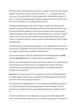
What’s the meaning of such a graph? It can be viewed as a “program” (therefore the name “branching program”) that computes a function f as follows. On an input x = x1…xn, the program starts at the source node. If the node is labeled by xi , then the program reads xi , and depending on whether xi = 0 and xi = 1, follows the corresponding edge. The program continues this way until it reaches to one of the two sinks, then outputs 0 or 1 according to the label of the sink. The length of a branching program is the number of edges in a longest path.If the nodes can be arranged into a sequence of levels with edges going only from one level to the next, then the width is the number of nodes of the largest level.(One can always add dummy nodes to make this happen without increasing the number of edges much.) Width corresponds to space, and length corresponds to time. If all nodes in the same level are labeled by the same variable, then the program is called oblivious. Our algorithm for the Parity function means that it can be computed by a width-2, length-n branching program. So branching programs are like decision tree algorithms (i.e. query algorithms) that we learned in the previous lecture. The difference is that if we have a bound for the width of a branching program, then we essentially consider decision tree algorithms with the space limit. Now one natural question is: What’s the computational power of branching programs of constant width and polynomial length? (For a concrete example, can it compute Majority?) Intuitively, this kind of program doesn’t look powerful since the constant width is a bottleneck of how much information can be carried in the process of computation. Most researchers had indeed conjectured that it cannot compute functions such as Majority. Thus the following theorem by Barrington came as a big surprise. Theorem 1.2. If a Boolean function f can be computed by polynomial-size {AND,OR} formula on xi’s and their negations, then it can also be computed by a branching program of polynomial length and width 5. (What’s more, the program is oblivious.) We can actually prove something stronger: If f can be computed by a {AND,OR} circuit of depth d, then it can be computed by an oblivious branching program of width 5 and length 4d . (Then for formula of size s, its depth is at most d = log2(s), so the branching program is of length at most 4d = s 2 .) We want to simulate the circuit. By de Morgan rule, it’s enough to simulate the negation and the (binary) AND gate. (It doesn’t change the size of a circuit much by stretching out an AND gate with

fanin more than 2 by inserting some AND gates with fanin 2.)To this end,Barrington observed that a special kind of branching programs are particular good:the computation from each level to the next is just a permutation.Namely,for a level in an oblivious branching program,suppose it reads xi,then the state transfer is from j to o(j)for some permutation o of (1,2,3,4,5).Note that o dependson xi, namely there are two permutation oo ando,to be applied.Consider a program P,which readsx,.., xi in that order.For notational convenience,denote the level-t permutation on input x by o(x)We say that P t-computes f if for all possible inputsx, fx)=1→(x).X)=t, fx)=0→oxd.c(x)=e, where e is the identity permutation(i.e.doing nothing). What's good for this kind of branching programs? Property 1.If Pt-computes f,then there is a branching program P't-computing-f,and P'has the same width and length as P. The reason is simple:Just replace the last step permutation o by o. Property 2.If P o-computes f and Q t-computes g,then there is a branching program oflength 2(length(P)+length(Q))which(oro)-computing fng The existence is given by Fig 1,which shows that ote,and ifeither o=e or t=e,then oto =e.This implies that the large branching program indeed computes fAg:if either for gevaluates to 0, then by definition of P and Q,we know that o=e or t=e,then oro=e.If both f and gevaluate to 1,then the large branching program always gives permutation(oto),which is not e. p=oto-lt-it-1 Fig 1.Barrington's permutations

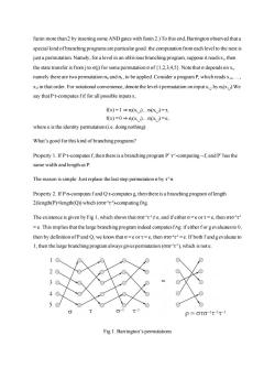
fanin more than 2 by inserting some AND gates with fanin 2.) To this end, Barrington observed that a special kind of branching programs are particular good: the computation from each level to the next is just a permutation. Namely, for a level in an oblivious branching program, suppose it reads xi , then the state transfer is from j to σ(j) for some permutation σ of {1,2,3,4,5}. Note that σ depends on xi , namely there are two permutation σ0 and σ1, to be applied. Consider a program P, which reads xi1, …, xil in that order. For notational convenience, denote the level-t permutation on input xi_t by σt(xi_t) We say that P τ-computes f if for all possible inputs x, f(x) = 1 ⇒ σl(xi_l)…σl(xi_l) = τ, f(x) = 0 ⇒ σl(xi_l)…σl(xi_l) = e, where e is the identity permutation (i.e. doing nothing). What’s good for this kind of branching programs? Property 1. If P τ-computes f, then there is a branching program P’ τ -1 -computing f, and P’ has the same width and length as P. The reason is simple: Just replace the last step permutation σ by τ -1σ. Property 2. If P σ-computes f and Q τ-computes g, then there is a branching program of length 2(length(P)+length(Q)) which (στσ -1 τ -1 )-computing f∧g. The existence is given by Fig 1, which shows that στσ -1 τ -1≠ e, and if either σ = e or τ = e, then στσ -1 τ -1 = e. This implies that the large branching program indeed computes f∧g: if either f or g evaluates to 0, then by definition of P and Q, we know that σ = e or τ = e, then στσ -1 τ -1 = e. If both f and g evaluate to 1, then the large branching program always gives permutation (στσ -1 τ -1 ), which is not e. Fig 1. Barrington’s permutations

With these two properties,we can prove the theorem by induction on d.Note that by de Morgan's rule, one can assume that the top gate is AND.So using the second property,the size blow up by a factor of 4 Finally,to use such a t-pemmutation branching program to compute f,one can just let the source be any ion the first level with t(i)i.Since te,such imust exist.Let the node t(i)on the last level by the 1-sink,and all other nodes links to a 0-sink. Finally let's come back to the original question of Majority function.It remains to show that Majority can be computed by a formula of polynomial size.This is indeed true;actually Valiant showed in [Val84]that it can be computed by a monotone formula of size O(n3.3). 2.From perfect matching to PIT and Circuit complexity 2.1 Bipartite perfect matching. Consider the following problem.Given an(n,n)-bipartite graph,decide whether it has a perfect matching.(Recall that a perfect matching is a permutation t s.t.every (i,(i))is an edge.) From the algorithm course,we know that the problem can be solved by transforming it into a max-flow problem.Here we present another algorithm which is more efficient for parallel computing. We associate an n-by-n matrix MG to the input graph G.The (i j)-entry of the matrix is xii if(i,j)EE, and 0 otherwise.By the definition of determinant,we have the following observation. Observation.Det(MG)is a zero polynomial if and only if G has a perfect matching. So to decide whether G has a perfect matching,it's sufficient to decide whether Det(MG)is a zero polynomial.Though this doesn't seem to be an easy job either,there is a very simple polynomial-time randomized algorithm based on the following famous lemma. Schwartz-Zippel Lemma.For any nonzero polynomial p(x1,...,x)over field F,if we pick n random elements ai,.,an from a subset S of F,Pr[p(a,.,an)=0]sdeg(p)/Sl. The lemma can be easily proven by induction on the deg(p);for an explicit proof,see the wiki page. In our bipartite matching problem,note that Det(MG)is a polynomial of variablesxi,and its degree is at most n.So we can just pick any field F ofsize,say,about n2,and pick random elements a,an from it.(Recall that for any N,there is a prime number p in [N,2N).So we can just pick F=Zp with p in [n2,2n2).Then let S=F.)Evaluate Det(MG)on(a1,..,an)to see whether it's 0.(Recall the fact that

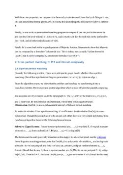
With these two properties, we can prove the theorem by induction on d. Note that by de Morgan’s rule, one can assume that the top gate is AND. So using the second property, the size blow up by a factor of 4. Finally, to use such a τ-permutation branching program to compute f, one can just let the source be any i on the first level with τ(i) ≠ i. Since τ ≠ e, such i must exist. Let the node τ(i) on the last level by the 1-sink, and all other nodes links to a 0-sink. Finally let’s come back to the original question of Majority function. It remains to show that Majority can be computed by a formula of polynomial size. This is indeed true; actually Valiant showed in [Val84] that it can be computed by a monotone formula of size O(n5.3). 2. From perfect matching to PIT and Circuit complexity 2.1 Bipartite perfect matching. Consider the following problem. Given an (n,n)-bipartite graph, decide whether it has a perfect matching. (Recall that a perfect matching is a permutation τ s.t. every (i, τ(i)) is an edge.) From the algorithm course, we know that the problem can be solved by transforming it into a max-flow problem. Here we present another algorithm which is more efficient for parallel computing. We associate an n-by-n matrix MG to the input graph G. The (i,j)-entry of the matrix is xij if (i,j)∈E, and 0 otherwise. By the definition of determinant, we have the following observation. Observation. Det(MG) is a zero polynomial if and only if G has a perfect matching. So to decide whether G has a perfect matching, it’s sufficient to decide whether Det(MG) is a zero polynomial. Though this doesn’t seem to be an easy job either, there is a very simple polynomial-time randomized algorithm based on the following famous lemma. Schwartz-Zippel Lemma. For any nonzero polynomial p(x1, …, xn) over field F, if we pick n random elements a1, .., an from a subset S of F, Pr[p(a1, .., an) = 0] ≤ deg(p)/|S|. The lemma can be easily proven by induction on the deg(p); for an explicit proof, see the wiki page. In our bipartite matching problem, note that Det(MG) is a polynomial of variables xij, and its degree is at most n. So we can just pick any field F of size, say, about n 2 , and pick random elements a1, .., an from it. (Recall that for any N, there is a prime number p in [N,2N). So we can just pick F = Zp with p in [n2 , 2n2 ). Then let S = F.) Evaluate Det(MG) on (a1, .., an) to see whether it’s 0. (Recall the fact that

determinent is easy to compute.)If it's 0,then claim that G doesn't have a perfect matching; otherwise claim that G does If G doesn't have a perfect matching,then Det(MG)is a zero polynomial,so whatever(a,..,an)is picked,the algorithm gives the correct answer.If G has a perfect matching,then Det(MG)is a nonzero polynomial,thus by the lemma,a random(a,..,a)is not the root with probability 1-1/n,thus the algorithm outputs the correct answer with high probability. 2.2 Arithmetic circuits and Polynomial ldentity Testing In the previous discussion,we ran into the problem of deciding whether a given polynomial is zero polynomial.This problem is very important on its own,and in this section we will discuss it in the framework of arithmetic circuits.An arithmetic circuit is similar to a Boolean circuit,except to use x and gates instead of AND and OR gates.More precisely,an arithmetic circuit over the field F and the set of variablesx={x1,...,x)is a directed acyclic graph (DAG),with each vertex having in-degree either 0 or 2.Each vertex with in-degree 0 is associated with either a variable from x or a field element from F.Each vertex with in-degree 2 is associated with either a x gate,or a gate. The size of a circuit is the number ofedges.The depth of a circuit is the number ofedges on a longest directed path.(There is one catch here:Sometimes people talk about constant-depth circuits,in which case there is no bound on the in-degree. An arithmetic circuit is an arithmetic formula if the DAG is a tree with the in-degree-0 gates being the leaves. An arithmetic circuit computes a polynomial in a natural way by following the direction of the graph and computation on the gates. Formally,the problem is defined as follows. Problem(Polynomial Identity Testing,or PIT)Given an arithmetic circuit,decide whether it computes the zero polynomial. Note that a polynomial is zero if and only if all its coefficients are zero.It's different than zero as a function,namely zero for all inputs.For example,x2-x takes zero values for all possible x in (0,1), but it's not a zero polynomial

determinent is easy to compute.) If it’s 0, then claim that G doesn’t have a perfect matching; otherwise claim that G does. If G doesn’t have a perfect matching, then Det(MG) is a zero polynomial, so whatever (a1, .., an) is picked, the algorithm gives the correct answer. If G has a perfect matching, then Det(MG) is a nonzero polynomial, thus by the lemma, a random (a1, .., an) is not the root with probability 1-1/n, thus the algorithm outputs the correct answer with high probability. 2.2 Arithmetic circuits and Polynomial Identity Testing In the previous discussion, we ran into the problem of deciding whether a given polynomial is zero polynomial. This problem is very important on its own, and in this section we will discuss it in the framework of arithmetic circuits. An arithmetic circuit is similar to a Boolean circuit, except to use × and + gates instead of AND and OR gates. More precisely, an arithmetic circuit Φ over the field F and the set of variables x = {x1, . . . , xn} is a directed acyclic graph (DAG), with each vertex having in-degree either 0 or 2. Each vertex with in-degree 0 is associated with either a variable from x or a field element from F. Each vertex with in-degree 2 is associated with either a ×gate, or a + gate. The size of a circuit is the number of edges. The depth of a circuit is the number of edges on a longest directed path. (There is one catch here: Sometimes people talk about constant-depth circuits, in which case there is no bound on the in-degree.) An arithmetic circuit is an arithmetic formula if the DAG is a tree with the in-degree-0 gates being the leaves. An arithmetic circuit computes a polynomial in a natural way by following the direction of the graph and computation on the gates. Formally, the problem is defined as follows. Problem (Polynomial Identity Testing, or PIT) Given an arithmetic circuit, decide whether it computes the zero polynomial. Note that a polynomial is zero if and only if all its coefficients are zero. It’s different than zero as a function, namely zero for all inputs. For example, x2 -x takes zero values for all possible x in {0,1}, but it’s not a zero polynomial

We can use Schwartz-Zippel Lemma to give a randomized polynomial-time algorithm for PIT.The real question is whether we have a deterministic polynomial-time algorithm.In complexity language, we know that PIT is in BPP,and wonder whether it's also in P. A nice (and recent)survey on arithmetic circuit complexity is [SY09],where you canalso find positive and negative results on algorithms for PI'T. References [LZ77]Richard J.Lipton and Yechezkel Zalcstein,Word Problems Solvable in Logspace,Journal ofthe ACM,1977. [SY09]Amir Shpilka and Amir Yehudayoff,Arithmetic Circuits:A Survey of Recent Results and Open Questions,Foundations and Trends in Theoretical Computer Science,Vol.5,Nos.3-4,207- 388,2009 [Val84]Leslie Valiant.Short monotone formulae for the majority function.Journal ofAlgorithms 5(3)363-366,1984

We can use Schwartz-Zippel Lemma to give a randomized polynomial-time algorithm for PIT. The real question is whether we have a deterministic polynomial-time algorithm. In complexity language, we know that PIT is in BPP, and wonder whether it’s also in P. A nice (and recent) survey on arithmetic circuit complexity is [SY09], where you can also find positive and negative results on algorithms for PIT. References [LZ77] Richard J. Lipton and Yechezkel Zalcstein, Word Problems Solvable in Logspace, Journal of the ACM, 1977. [SY09] Amir Shpilka and Amir Yehudayoff , Arithmetic Circuits: A Survey of Recent Results and Open Questions, Foundations and Trends in Theoretical Computer Science, Vol. 5, Nos. 3–4, 207– 388, 2009. [Val84] Leslie Valiant. Short monotone formulae for the majority function. Journal of Algorithms 5 (3): 363–366, 1984