香港中文大学:《Theory of Computational Complexity》课程教学资源(讲义)Lecture 10 Circuit Complexity 2

Lecture 10.Circuit Complexity 2 In last lecture we proved exponential lower bound for depth-3 circuit.The method doesn't extend to larger depth.In this lecture,we show how to prove exponential lower bounds for constant-depth circuits. 1.DNF,CNF,and Switching Lemma Recall: CNF:f)=where each is a literal,and each V is a clause. The function f is called a k-CNF if each ki s k. DNF:f(-Vwhere each is a monomial.The function f is called a k-DNF if each ki k. In general,a k-CNF is not necessarily also a k-DNF.For example,the AND function is a 1-CNF,but an n-DNF.The Switching Lemma says that if we fix some variables of a t-CNF, then we obtain a subfunction which is an s-DNF for some small s.We can actually use a random restriction.A p-random restriction makes each bit unfixed with probability p,and fixed with probability 1-p.In the latter case,the bit is fixed to be 0 or 1 each equal probability.We use p to denote a random restriction,and fo the resulting subfunction.The following lemma was given by Hastad [Has89]. Lemma 1.1.If f is a t-CNF,and p is a p-random restriction,then Pr[fo can be written as an s-DNF]1-(5pt)s. The original proof uses probabilistic arguments.Also see Razborov's elegent proof [Raz95] using a combinatorial method. Recall that deg(f)is the degree of the function represented as a polynomial in x,,n over R.Equivalently,it is the largest max{ISl:f(s)0}where the numbers f(s)are the Fourier coefficients
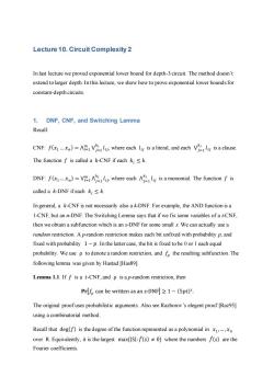
Lecture 10. Circuit Complexity 2 In last lecture we proved exponential lower bound for depth-3 circuit. The method doesn’t extend to larger depth. In this lecture, we show how to prove exponential lower bounds for constant-depth circuits. 1. DNF, CNF, and Switching Lemma Recall: CNF: 𝑓(𝑥1 … 𝑥𝑛 ) = ⋀ ⋁ 𝑙 𝑖𝑗 𝑘𝑖 𝑗=1 𝑚 𝑖=1 , where each 𝑙 𝑖𝑗 is a literal, and each ⋁ 𝑙 𝑖𝑗 𝑘𝑖 𝑗=1 is a clause. The function 𝑓 is called a 𝑘-CNF if each 𝑘𝑖 ≤ 𝑘. DNF: 𝑓(𝑥1 … 𝑥𝑛 ) = ⋁ ⋀ 𝑙 𝑖𝑗 𝑘𝑖 𝑗=1 𝑚 𝑖=1 , where each ⋀ 𝑙 𝑖𝑗 𝑘𝑖 𝑗=1 is a monomial. The function 𝑓 is called a 𝑘-DNF if each 𝑘𝑖 ≤ 𝑘. In general, a 𝑘-CNF is not necessarily also a k-DNF. For example, the AND function is a 1-CNF, but an n-DNF. The Switching Lemma says that if we fix some variables of a t-CNF, then we obtain a subfunction which is an s-DNF for some small s. We can actually use a random restriction. A p-random restriction makes each bit unfixed with probability p, and fixed with probability 1 − 𝑝. In the latter case, the bit is fixed to be 0 or 1 each equal probability. We use ρ to denote a random restriction, and 𝑓𝜌 the resulting subfunction. The following lemma was given by Hastad [Has89]. Lemma 1.1. If 𝑓 is a 𝑡-CNF, and ρ is a p-random restriction, then 𝐏𝐫[𝑓𝜌 can be written as an 𝑠-DNF] ≥ 1 − (5𝑝𝑡) 𝑠 . The original proof uses probabilistic arguments. Also see Razborov’s elegent proof [Raz95] using a combinatorial method. Recall that deg(𝑓) is the degree of the function represented as a polynomial in 𝑥1 ,…, 𝑥𝑛 over R. Equivalently, it is the largest max{|S|: 𝑓̂(𝑠) ≠ 0} where the numbers 𝑓̂(𝑠) are the Fourier coefficients

We now give another lemma. Lemma 1.2.Under the condition of Lemma 1.1, Pr[deg(fo)>s]<(5pt)s, 2.Application of Switching Lemma Recall that certificate complexity of a function f:(0.1)"{0,1}on an input x is C(f,x)=min {ISl:Ss [nl,f(y)=f(x)Vy with ys =xs} where xs=(xi:iE S).Further define Ci(f)=max {C(f,x):f(x)=13,Co(f)=max {C(f,x):f(x)=03, and C(f)=maxC(f,x),Cmin (f)=min C(f,x). To get familiar with the concept,consider some specific functions: AND:Co(f)=1,Ci(f)=n,C(f)=n,Cmin (f)=1. OR:Co(f)=n,Ci(f)=1,C(f)=n,Cmin(f)=1. Parity:Co(f)=n,Ci(f)=n,C(f)=n,Cmin(f)=n. Majority:Co(f)=n/2,C1(f)=n/2,C(f)=n/2,Cmin (f)=n/2. Theorem 2.1.Iffcan be computed by a depth-(d +1)circuit of size S,then 1 Cmin(月≤n(1-100og时+21ogs. Using the parameters for Parity,we immed iately get the following corollary. Corollary.If a circuit with depth d computes the Parity function,then the circuit size is at least S=2n(n4-1)
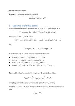
We now give another lemma. Lemma 1.2. Under the condition of Lemma 1.1, 𝐏𝐫[deg(𝑓𝜌 ) > 𝑠] < (5𝑝𝑡) 𝑠 , 2. Application of Switching Lemma Recall that certificate complexity of a function 𝑓:{0.1} 𝑛 → {0,1} on an input 𝑥 is 𝐶(𝑓, 𝑥) = min {|𝑆|: 𝑆 ⊆ [𝑛],𝑓(𝑦) = 𝑓(𝑥) ∀𝑦 with 𝑦𝑆 = 𝑥𝑆 } where 𝑥𝑆 = (𝑥𝑖 :𝑖 ∈ 𝑆). Further define 𝐶1 (𝑓) = max {𝐶(𝑓, 𝑥):𝑓(𝑥) = 1}, 𝐶0 (𝑓) = max {𝐶(𝑓,𝑥): 𝑓(𝑥) = 0}, and 𝐶(𝑓) = max 𝑥 𝐶(𝑓, 𝑥) , 𝐶𝑚𝑖𝑛(𝑓) = min 𝑥 𝐶(𝑓, 𝑥) . To get familiar with the concept, consider some specific functions: ⚫ AND: 𝐶0 (𝑓) = 1, 𝐶1 (𝑓) = 𝑛, 𝐶(𝑓) = 𝑛, 𝐶𝑚𝑖𝑛 (𝑓) = 1. ⚫ OR: 𝐶0 (𝑓) = 𝑛, 𝐶1 (𝑓) = 1, 𝐶(𝑓) = 𝑛, 𝐶𝑚𝑖𝑛(𝑓) = 1. ⚫ Parity: 𝐶0 (𝑓) = 𝑛, 𝐶1 (𝑓) = 𝑛, 𝐶(𝑓) = 𝑛, 𝐶𝑚𝑖𝑛(𝑓) = 𝑛. ⚫ Majority: 𝐶0 (𝑓) = 𝑛/2, 𝐶1 (𝑓) = 𝑛/2, 𝐶(𝑓) = 𝑛/2,𝐶𝑚𝑖𝑛 (𝑓) = 𝑛/2. Theorem 2.1. If f can be computed by a depth-(𝑑 + 1) circuit of size S, then 𝐶𝑚𝑖𝑛(𝑓) ≤ 𝑛 (1 − 1 10𝑑(log 𝑆) 𝑑−1 ) + 2 log 𝑆. Using the parameters for Parity, we immediately get the following corollary. Corollary. If a circuit with depth d computes the Parity function, then the circuit size is at least 𝑆 = 2 𝛺(𝑛 𝑑−1 )

Now we sketch the proof for Theorem 2.1. Proofidea (of Theorem 2.1).Repeatedly apply the Switching Lemma,in a bottom up manner, to reduce the depth.Use the lemma with s =t =2log S,and p =1/10s.Once we replace a CNF by a DNF,we'll see two consecutive layers of OR gates,thus we can collapse these two layers.Each round leaves about p-fraction of variables unfixed,thus finally we get a depth-2 circuit which computes a subfunction g of pn=n/(10log S)1variables.We need some special handling for the first step,which can also be done as an application of the switching lemma.And finally the s-DNF function g can be made constant by restricting s variables.Thus overall we restrictedngvariables and obtained a constant function.By definition of Cmin(f),we get the claimed statement. Next we show exponential lower bounds for more general functions,superseding the previous result for Parity.It's interesting also because it links circuit complexity and Fourier coefficients.This famous result was given in [LMN93]. Theorem 2.2.If a circuit with depth d and size Mcomputes a function f:{0,1)m{-1,+1), then M≥2ak4.∑.f92. s:Isl>k Note that for Parity function,there is only one nonzero Fourier coefficient:f(1")=1.Thus we can take k=n-1 and obtain a lower bound of 2(n) We'll need a couple of lemmas to prove this theorem. Lemma2.3.∑t:f(t)2≤2Esup[Et:ltsl-pk/2f()2] Proof.Think of T also as a random variable distributed according to Fourier weights f(t)2 (We identify a string s E{0,1)m with a subset S[n].)Then RHS =2 Es[Pr[IT n SI >pk/2]]=2 Pr[IT nSI pk/2]
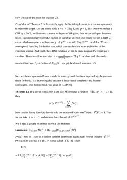
Now we sketch the proof for Theorem 2.1. Proof idea (of Theorem 2.1). Repeatedly apply the Switching Lemma, in a bottom up manner, to reduce the depth. Use the lemma with 𝑠 = 𝑡 = 2log 𝑆, and 𝑝 = 1/10𝑠. Once we replace a CNF by a DNF, we’ll see two consecutive layers of OR gates, thus we can collapse these two layers. Each round leaves about p-fraction of variables unfixed, thus finally we get a depth-2 circuit which computes a subfunction 𝑔 of 𝑝 𝑑−1 𝑛 = 𝑛/(10log 𝑆) 𝑑−1 variables. We need some special handling for the first step, which can also be done as an application of the switching lemma. And finally the s-DNF function 𝑔 can be made constant by restricting 𝑠 variables. Thus overall we restricted 𝑛 − 𝑛 10𝑑 (log 𝑆)𝑑−1 + 2log 𝑆 variables and obtained a constant function. By definition of 𝐶𝑚𝑖𝑛(𝑓), we get the claimed statement. □ Next we show exponential lower bounds for more general functions, superseding the previous result for Parity. It’s interesting also because it links circuit complexity and Fourier coefficients. This famous result was given in [LMN93]. Theorem 2.2. If a circuit with depth d and size M computes a function 𝑓:{0,1} 𝑛 → {−1, +1}, then 𝑀 ≥ 2 Ω(𝑘 1/𝑑 ) ⋅ ∑ 𝑓̂(𝑠) 2 𝑠:|𝑠|>𝑘 . Note that for Parity function, there is only one nonzero Fourier coefficient: 𝑓̂(1 𝑛) = 1. Thus we can take 𝑘 = 𝑛 − 1 and obtain a lower bound of 2 Ω(𝑛 1/𝑑 ) . We’ll need a couple of lemmas to prove this theorem. Lemma 2.3. ∑ 𝑓̂(𝑡) 2 𝑡:|𝑡|>𝑘 ≤ 2E𝑠←𝜇(𝑝) [∑ 𝑓̂(𝑡) 2 𝑡:|𝑡𝑆 |>𝑝𝑘/2 ]. Proof. Think of T also as a random variable distributed according to Fourier weights 𝑓̂(𝑡) 2 . (We identify a string 𝑠 ∈ {0,1} 𝑛 with a subset 𝑆 ⊆ [𝑛].) Then RHS = 2 E𝑆 [Pr 𝑇 [|𝑇 ∩ 𝑆| > 𝑝𝑘/2]] = 2 Pr 𝑆,𝑇 [|𝑇 ∩ 𝑆| > 𝑝𝑘/2]

=2(PrIT>P-TnSI>pk/2IIT>k]+Pr[ITI≤k]Pr[lT nSl>pk/2IITI≤k]) 22 Pr[ITI k]Pr[lT n Sl pk/2 I ITI>k] >2Pr[ITI>k](1/2) Pr[IT n Sl pk/2I ITI>k]>1/2 by Chernoff Pr[ITI>k] =LHS 0 Lemma2.4 Suppose that Sn]with S=1.By r ES we mean to draw r from (0.1s uniformly at random. 1.For any fired ts,f(t)2=Eresf(ts)2 2.∑(t2=E,es∑sf(ts)]≤Pr,edeg(fr)>I. Proof 1. ∑foP=∑(Eesk.ts)its)°=∑(E.cslx.sxts)is)ts =Eres[(∑七(s)x.(ts)f元ts)fts) -E.esj-(ts)j(ts)-Eres[j-(ts)] 2.By the above result, ∑ft2=∑E,eslf-(ts)]=Ees∑ftsP] t:Its >l ts:ts ts:ts> For the second part:For a function f,denote by W>t the sum of Fourier coefficients f(s)with s>l.that E,es[∑ts月] ts:ts> =Pr[deg(f)IEW>(f)I deg(f)+Pr[deg(f)>E[w(f)I deg(f)> =Pr[deg(f)>IE[W>(f)I deg(f)> ≤Pr[deg(fn)>I where the second step is because EW(f)deg(f)<1]=0 by definition of deg
= 2 (Pr T [|𝑇| > 𝑘] Pr S [|𝑇 ∩ 𝑆| > 𝑝𝑘/2| |𝑇| > 𝑘] + Pr 𝑇 [|𝑇| ≤ 𝑘] Pr 𝑆 [|𝑇 ∩ 𝑆| > 𝑝𝑘/2| |𝑇| ≤ 𝑘]) ≥ 2 Pr T [|𝑇| > 𝑘] Pr 𝑆 [|𝑇 ∩ 𝑆| > 𝑝𝑘/2 | |𝑇| > 𝑘] > 2 Pr 𝑇 [|𝑇| > 𝑘] (1/2) ( Pr 𝑆 [|𝑇 ∩ 𝑆| > 𝑝𝑘/2 | |𝑇| > 𝑘] > 1/2 by Chernoff ) = Pr 𝑇 [|𝑇| > 𝑘] = LHS □

Lemma 2.5.A p-random restriction p gives a subfunction fo of deg(f)sl with probability at least 1-M2-.Here p This can be proven by a similar argument as in the proof of Theorem 2.1;one just need to use Lemma 1.2 instead of Lemma 1.1.See [LMN93]for details. Proofof Theorem 2.2.Let u(p)be the distribution on (0,1)by setting each coordinate to be 1 with probability p.Let p=1/(10k(d-1)/d),I=pk/2=k/4/20.Note that we identify a string s E [0,1)n and a subset Ss[n]. ∑t:lekf()2≤2Es-u()s>pk/2f()] (Lemma 2.3) ≤2Es-up)[Pr[degf)>] (Lemma 2.4) ≤2M2-l (Lemma 2.5) 口 References [Has89]J.Hastad,Almost optimal lower bounds for small depth circuits,Advances in Computing Research,vol.5,pp.143-170,1989 Raz95]A.A.Razborov,Bounded arithmetics and lower bounds in boolean complexity, in Proceedings of Workshop on Feasible Mathematics II,1995 [LMN93]N.Linial,Y.Mansour,and N.Nisan,Constant depth circuits,Fourier transforms and learnability,Journal of the ACM,vol.40,pp.607-620,1993
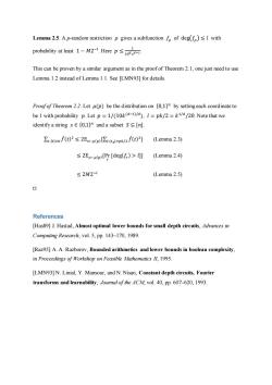
Lemma 2.5. A p-random restriction 𝜌 gives a subfunction 𝑓𝜌 of deg(𝑓𝜌 ) ≤ 𝑙 with probability at least 1 − 𝑀2 −𝑙 . Here 𝑝 ≤ 1 10𝑑 𝑠 𝑑−1 . This can be proven by a similar argument as in the proof of Theorem 2.1; one just need to use Lemma 1.2 instead of Lemma 1.1. See [LMN93] for details. Proof of Theorem 2.2. Let 𝜇(𝑝) be the distribution on {0,1} 𝑛 by setting each coordinate to be 1 with probability 𝑝. Let 𝑝 = 1/(10𝑘 (𝑑−1)/𝑑 ), 𝑙 = 𝑝𝑘/2 = 𝑘 1/𝑑 /20. Note that we identify a string 𝑠 ∈ {0,1} 𝑛 and a subset 𝑆 ⊆ [𝑛]. ∑ 𝑓̂(𝑡) 2 𝑡:|𝑡|>𝑘 ≤ 2E𝑠←𝜇(𝑝) [∑ 𝑓̂(𝑡) 2 𝑡:|𝑡𝑆 |>𝑝𝑘/2 ] (Lemma 2.3) ≤ 2E𝑠←𝜇(𝑝) [Pr r [deg(𝑓𝑟 ) > 𝑙]] (Lemma 2.4) ≤ 2𝑀2 −𝑙 (Lemma 2.5) □ References [Has89] J. Hastad, Almost optimal lower bounds for small depth circuits, Advances in Computing Research, vol. 5, pp. 143–170, 1989. [Raz95] A. A. Razborov, Bounded arithmetics and lower bounds in boolean complexity, in Proceedings of Workshop on Feasible Mathematics II, 1995. [LMN93] N. Linial, Y. Mansour, and N. Nisan, Constant depth circuits, Fourier transforms and learnability, Journal of the ACM, vol. 40, pp. 607–620, 1993
按次数下载不扣除下载券;
注册用户24小时内重复下载只扣除一次;
顺序:VIP每日次数-->可用次数-->下载券;
- 香港中文大学:《Theory of Computational Complexity》课程教学资源(讲义)Lecture 9 Circuit Complexity.docx
- 香港中文大学:《Theory of Computational Complexity》课程教学资源(讲义)Lecture 7 Decision Tree Complexity and Fourier analysis.docx
- 香港中文大学:《Theory of Computational Complexity》课程教学资源(讲义)Lecture 6 Formula complexity II.docx
- 香港中文大学:《Theory of Computational Complexity》课程教学资源(讲义)Lecture 5 Formula complexity I.docx
- 香港中文大学:《Theory of Computational Complexity》课程教学资源(讲义)Lecture 4 Multiparty Communication Complexity.docx
- 香港中文大学:《Theory of Computational Complexity》课程教学资源(讲义)Lecture 3 Communication complexity.docx
- 香港中文大学:《Theory of Computational Complexity》课程教学资源(讲义)Lecture 2 More samples.docx
- 香港中文大学:《Theory of Computational Complexity》课程教学资源(讲义)Lecture 1 Samples of possibility and impossibility results in algorithm designing.docx
- 香港中文大学:《Design and Analysis of Algorithms》课程教学资源(辅导课件)tutorial 09.pptx
- 香港中文大学:《Design and Analysis of Algorithms》课程教学资源(辅导课件)tutorial 08.pptx
- 香港中文大学:《Design and Analysis of Algorithms》课程教学资源(辅导课件)tutorial 06.pptx
- 香港中文大学:《Design and Analysis of Algorithms》课程教学资源(辅导课件)tutorial 05.pptx
- 香港中文大学:《Design and Analysis of Algorithms》课程教学资源(辅导课件)tutorial 04.pptx
- 香港中文大学:《Design and Analysis of Algorithms》课程教学资源(辅导课件)tutorial 03.pptx
- 香港中文大学:《Design and Analysis of Algorithms》课程教学资源(辅导课件)tutorial 02.pptx
- 香港中文大学:《Design and Analysis of Algorithms》课程教学资源(辅导课件)tutorial 12.pptx
- 香港中文大学:《Design and Analysis of Algorithms》课程教学资源(辅导课件)tutorial 11.pptx
- 香港中文大学:《Design and Analysis of Algorithms》课程教学资源(辅导课件)tutorial 10.pptx
- 香港中文大学:《Design and Analysis of Algorithms》课程教学资源(辅导课件)tutorial 01.pptx
- 香港中文大学:《Design and Analysis of Algorithms》课程教学资源(PPT课件讲稿)Week 10 Stable Matching and Secretary Problem.pptx
- 香港中文大学:《Theory of Computational Complexity》课程教学资源(讲义)Lecture 11 Information theoretical argument.docx
- 香港中文大学:《Theory of Computational Complexity》课程教学资源(讲义)Lecture 12 A glimpse of computational complexity.docx
- 香港中文大学:《CMSC5719 Seminar》课程教学资源(讲义)Lecture 08 An introduction to expander graphs(EXPANDER GRAPHS AND THEIR APPLICATIONS).pdf
- 香港中文大学:《CMSC5719 Seminar》课程教学资源(讲义)Lecture 01 A Secure Overlay Cloud Storage System with Access Control and Assured Deletion.pdf
- 香港中文大学:《CMSC5719 Seminar》课程教学资源(讲义)Lecture 02 Game theory in computer science.pptx
- 香港中文大学:《CMSC5719 Seminar》课程教学资源(讲义)Lecture 03 Controlling Salinity in a Potable Water Supply System Using a Constraint Programming Approach.pdf
- 香港中文大学:《CMSC5719 Seminar》课程教学资源(讲义)Lecture 04 CRYPTOGRAPHY.pptx
- 香港中文大学:《CMSC5719 Seminar》课程教学资源(讲义)Lecture 05 Fault-Tolerant Computing.ppt
- 香港中文大学:《CMSC5719 Seminar》课程教学资源(讲义)Lecture 06 3D computer vision techniques.ppt
- 香港中文大学:《CMSC5719 Seminar》课程教学资源(讲义)Lecture 07-1 Research and Applications of Virtual Medicine Part I Introduction to Medical Visualization.pdf
- 香港中文大学:《CMSC5719 Seminar》课程教学资源(讲义)Lecture 07-2 Research and Applications of Virtual Medicine Part II Virtual Reality Based Surgical Simulations.pdf
- 香港中文大学:《CMSC5719 Seminar》课程教学资源(讲义)Lecture 11 Design of Microfluidics-Based Biochips.pdf
- 香港中文大学:《CMSC5719 Seminar》课程教学资源(讲义)Lecture 10 An Introduction to Bioinformatics and its application in Protein-DNA/Protein Interactions Research and Drug Discovery.pptx
- 香港中文大学:《CMSC5719 Seminar》课程教学资源(讲义)Lecture 12 Introduction to Computational Photography.ppt
- Minimal Cover-Automata for Finite Languages.pdf
- 香港中文大学:《Topics in Theoretical Computer Science》课程教学资源(PPT课件讲稿)Lecture 7 Stable matching.Gale-Shapley algorithm.pptx
- 《农业信息技术概论》课程教学资源(教学大纲).pdf
- 《仿真与虚拟农业》课程教学资源(实验指导).pdf
- 天津农学院:《微机原理与汇编语言程序设计》课程教学资源(实验指导书).pdf
- 《3S技术导论》课程教学资源(实验指导).pdf
