同济大学：《传播信道特征估计和建模》课程教案讲义（射线追踪）01 Deterministic radio propagation modeling and ray tracing - Introduction to deterministic propagation modelling

Alma Mater Studiorum-DEI Deterministic radio propagation modeling and ray tracing Vittorio Degli-Esposti Alma Mater Studiorum-University of Bologna,Italy Department of Electrical,Electronic and Information Engineering(DEl)

Alma Mater Studiorum – DEI Deterministic radio propagation modeling and ray tracing Vittorio Degli-Esposti Alma Mater Studiorum - University of Bologna, Italy Department of Electrical, Electronic and Information Engineering (DEI)

Course outline 1) Introduction to deterministic propagation modelling 2) Geometrical Theory of Propagation I-The ray concept-Reflection and transmission 3) Geometrical Theory of Propagation II-Diffraction,multipath 4) Ray Tracing I 5) Ray Tracing II-Diffuse scattering modelling 6) Deterministic channel modelling I 7) Deterministic channel modelling II-Examples 8) Project -discussion 4

4 1) Introduction to deterministic propagation modelling 2) Geometrical Theory of Propagation I - The ray concept – Reflection and transmission 3) Geometrical Theory of Propagation II - Diffraction, multipath 4) Ray Tracing I 5) Ray Tracing II – Diffuse scattering modelling 6) Deterministic channel modelling I 7) Deterministic channel modelling II – Examples 8) Project - discussion Course outline

Course info 。 Slides and material available at There will be updates during the course Please print slides and take notes aside A"Project"will be assigned based on course content and exercises Last lesson will be on project correction and discussion 5

5 Course info • Slides and material available at … • There will be updates during the course • Please print slides and take notes aside ! • A “Project” will be assigned based on course content and exercises • Last lesson will be on project correction and discussion

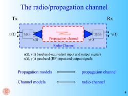
The radio/propagation channel Tx Rx u() MO DEM v(t) Propagation channel y(t) Radio Channel u(t),v(t)baseband-equivalent input and output signals x(t),y(t)passband(RF)input and output signals Propagation models propagation channel Channel models radio channel 6

The radio/propagation channel Tx Rx Propagation models propagation channel Channel models radio channel Radio Channel Propagation channel u(t) MO- DEM- v(t) x(t) y(t) u(t), v(t) baseband-equivalent input and output signals x(t), y(t) passband (RF) input and output signals 6

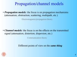
Propagation/channel models Propagation models:the focus is on propagation mechanisms (attenuation,obstruction,scattering,multipath,etc.) Electromagnetic/propagation theory Channel models:the focus is on the effects on the transmitted signal (attenuation,distortion,dispersion,etc.) Communication theory Different points of view on the same thing

7 Propagation/channel models • Propagation models: the focus is on propagation mechanisms (attenuation, obstruction, scattering, multipath, etc.) • Channel models: the focus is on the effects on the transmitted signal (attenuation, distortion, dispersion, etc.) Different points of view on the same thing Electromagnetic/propagation theory Communication theory

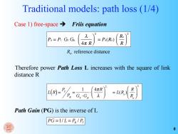
Traditional models:path loss (1/4) Case 1)free-space Friis equation 2 Px=Pr GrGR Ro 4πR =Px(Ro) R Ro reference distance Therefore power Path Loss L increases with the square of link distance R 4πR =L(R) R Path Gain (PG)is the inverse of L PG=1/L=PR/P 8

8 Traditional models: path loss (1/4) Case 1) free-space  Friis equation Therefore power Path Loss L increases with the square of link distance R L(R) = PT PR = 1 GT ⋅GR ⋅ 4πR λ ⎛ ⎝ ⎜ ⎞ ⎠ ⎟ 2 = L(R o ) R R o ⎛ ⎝ ⎜ ⎞ ⎠ ⎟ 2 Path Gain (PG) is the inverse of L 1/ / PG = L = PR PT PR = PT GT GR λ 4π R ⎛ ⎝ ⎜ ⎞ ⎠ ⎟ 2 = PR(R0) R0 R ⎛ ⎝ ⎜ ⎞ ⎠ ⎟ 2 Ro reference distance

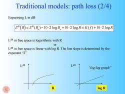
Traditional models:path loss (2/4) Expressing L in dB: L4R (R)=L4R (R)-10.2 logR+10.2 logR=K(f)+10.2 logR LdB in free space is logarithmic with R or LdB in free space is linear with log R.The line slope is determined by the exponent"2” LdB LdB “log-log graph'” log R

Expressing L in dB: LdB (R) = LdB (R o ) −10⋅2 log R o +10⋅2 log R = K( f ) +10⋅2 log R LdB in free space is logarithmic with R or LdB in free space is linear with log R. The line slope is determined by the exponent “2” LdB R LdB log R Traditional models: path loss (2/4) “log-log graph

Traditional models:path loss(3/4) Case 2)real environment> Hata-like models 40 L(1000) (R)=L(R,) R R。 2 100 Z(R)=K(f,)+10·a logR An attenuation law similar to free space is assumed but with a different exponent: a path loss exponent or path loss factor 0u>2 a is derived through fitting(regression line)on a set of measured path loss data →empirical modeling 10

10 An attenuation law similar to free space is assumed but with a different exponent: α path loss exponent or path loss factor α > 2 α is derived through fitting (regression line) on a set of measured path loss data  empirical modeling Traditional models: path loss (3/4) Case 2) real environment  Hata-like models LdB (R) = K( f ,α) +10⋅α log R L(R) = L(R o ) R R o ⎛ ⎝ ⎜ ⎞ ⎠ ⎟ α

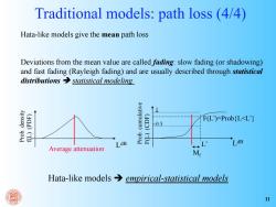
Traditional models:path loss (4/4) Hata-like models give the mean path loss Deviations from the mean value are called fading:slow fading (or shadowing) and fast fading (Rayleigh fading)and are usually described through statistical distributions statistical modeling (add)(T Bane nuno 'qold (ado)(Da F(L)=Prob L<L' 0.5 LdB LdB Average attenuation M Hata-like models→ empirical-statistical models 11

Hata-like models give the mean path loss Deviations from the mean value are called fading: slow fading (or shadowing) and fast fading (Rayleigh fading) and are usually described through statistical distributions  statistical modeling Average attenuation Prob. density f(L) (PDF) Prob. cumulative F(L) (CDF) LdB ~0.5 1 LdB F(L’)=Prob{L<L’} L’ Traditional models: path loss (4/4) Mf Hata-like models  empirical-statistical models 11

Other functional dependences of L However,in some cases not only achanges w.r.t.free space,but the overall functional dependance with R changes.Ex:indoors: Tx Rx office rooms L (R)=I4H (R)+IN=K+20logR- Multi-wall R model Ex:propagation through a lossy medium Specific attenuation [dB/m] L(R=L(R+[dBIm·R Linear model 12

12 However, in some cases not only αchanges w.r.t. free space, but the overall functional dependance with R changes. Ex: indoors: Tx Rx office rooms LdB (R) = L 0 dB (R) + L W dB ⋅ NW = K + 20log R + L W dBNW R ⎛ ⎝ ⎜ ⎜ ⎞ ⎠ ⎟ ⎟ ⋅ R Specific attenuation [dB/m] Other functional dependences of L Ex: propagation through a lossy medium LdB (R) = L 0 dB (R) + α S R [dB / m]⋅ R Tx Rx Multi-wall model Linear model