电子科技大学：《数字信号处理 Digital Signal Processing》课程教学资源（课件讲稿）Chapter 06 Digital Filter Structures

Chapter 6 Digital Filter Structures

Chapter 6 Digital Filter Structures

Ha() Ha() 1+δ 1+e2 -Passband- Stopband- Passband- Stopband- 2 p Qs 0 s - Transition Transition band band ·2p-passband edge ·1/V(1+ε2)-Maximum frequency passband deviation ·2s-stopband edge frequency 1/A Maximum stopband ·δp-peak ripple magnitude value in the passband ·δs-peak ripple Transition ratio k=p/s value in the stopband k1=ε/V(A2-1)

• 1 / √(1 + ε2) - Maximum passband deviation • 1/A - Maximum stopband magnitude • Transition ratio k = Ωp/ Ωs • k1 = ε/ √(A2 -1) • Ωp - passband edge frequency • Ωs - stopband edge frequency • δp - peak ripple value in the passband • δs - peak ripple value in the stopband

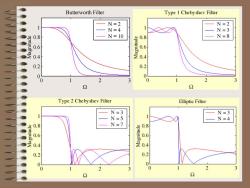
Butterworth Filter Type 1 Chebyshev Filter N=2 N=2 N=4 N=3 N=10 0.8 N=8 0.6 0.4 0.2 0.2 0 2 3 0 2 2 2 Type 2 Cheby shev Filter Elliptic Filter N=3 N=3 N=5 N=4 0.8 N=7 0.8 opmuew 0.6 0.6 0.4 0.4 0.2 0.2 0 2 3 0 2 3

0 1 2 3 0 0.2 0.4 0.6 0.81 Ω Magnitude Butterworth Filter N = 2 N = 4 N = 10

§6.1 Introduction The convolution sum description of an LTI discrete-time system can,in principle,be used to implement the system For an IIR finite-dimensional system this approach is not practical as here the impulse response is of infinite length However,a direct implementation of the IIR finite-dimensional system is practical

• The convolution sum description of an LTI discrete-time system can, in principle, be used to implement the system • For an IIR finite-dimensional system this approach is not practical as here the impulse response is of infinite length • However, a direct implementation of the IIR finite-dimensional system is practical §6.1 Introduction

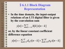
§6.l.1 Block Diagram Representation In the time domain,the input-output relations of an LTI digital filter is given by the convolution sum Hm=∑-hMk]n-k] or,by the linear constant coefficient difference equation [m=-∑1d[n-]+∑0Pkx[n-]

§6.1.1 Block Diagram Representation • In the time domain, the input-output relations of an LTI digital filter is given by the convolution sum ∑∞ =−∞ = − k y[n] h[k] x[n k] ∑ = ∑ = = − − + − M k k N k k y n d y n k p x n k 1 0 [ ] [ ] [ ] or, by the linear constant coefficient difference equation

§6.1.1 Block Diagram Representation For the implementation of an LTI digital filter, the input-output relationship must be described by a valid computational algorithm To illustrate what we mean by a computational algorithm,consider the causal first-order LTI digital filter shown below x y[n]

§6.1.1 Block Diagram Representation • For the implementation of an LTI digital filter, the input-output relationship must be described by a valid computational algorithm • To illustrate what we mean by a computational algorithm, consider the causal first-order LTI digital filter shown below

§6.1.1 Block Diagram Representation Each step of the calculation requires a knowledge of the previously calculated value of the output sample (delayed value of the output),the present value of the input sample, and the previous value of the input sample (delayed value of the input) As a result,the first-order difference equation can be interpreted as a valid computational algorithm

§6.1.1 Block Diagram Representation • Each step of the calculation requires a knowledge of the previously calculated value of the output sample (delayed value of the output), the present value of the input sample, and the previous value of the input sample (delayed value of the input) • As a result, the first-order difference equation can be interpreted as a valid computational algorithm

S 6.1.2 Basic Building Blocks The computational algorithm of an LTI digital filter can be conveniently represented in block diagram form using the basic building blocks shown below x[n] wn] Multiplier Adder x(n] xInl yn] Unit delay Pick-off node

§6.1.2 Basic Building Blocks • The computational algorithm of an LTI digital filter can be conveniently represented in block diagram form using the basic building blocks shown below x[n] y[n] w[n] + A x[n] y[n] y[n] −1 x[n] z x[n] x[n] x[n] Adder Unit delay Multiplier Pick-off node

6.1.3 Analysis of Block Diagrams Carried out by writing down the expressions for the output signals of each adder as a sum of its input signals,and developing a set of equations relating the filter input and output signals in terms of all internal signals Eliminating the unwanted internal variables then results in the expression for the output signal as a function of the input signal and the filter parameters that are the multiplier coefficients

§6.1.3 Analysis of Block Diagrams • Carried out by writing down the expressions for the output signals of each adder as a sum of its input signals, and developing a set of equations relating the filter input and output signals in terms of all internal signals • Eliminating the unwanted internal variables then results in the expression for the output signal as a function of the input signal and the filter parameters that are the multiplier coefficients

6.2 Equivalent Structures Two digital filter structures are defined to be equivalent if they have the same transfer function We describe next a number of methods for the generation of equivalent structures However,a fairly simple way to generate an equivalent structure from a given realization is via the transpose operation

§6.2 Equivalent Structures • Two digital filter structures are defined to be equivalent if they have the same transfer function • We describe next a number of methods for the generation of equivalent structures • However, a fairly simple way to generate an equivalent structure from a given realization is via the transpose operation