香港中文大学：《Topics in Theoretical Computer Science》课程教学资源（PPT课件讲稿）Lecture 11 Influence maximization on social network

CMS57opomter ci Week 11:Influence Maximization on Social Networks Instructor:Shengyu Zhang

Instructor: Shengyu Zhang 1

Location change for the final 2 classes Nov 17:YIA 404 (Yasumoto International Academic Park康本國祭學術園) ■Nov24:No class. Conference leave. Dec 1:YIA 508 (Yasumoto International Academic Park康本國祭學術園) 2

Location change for the final 2 classes ◼ Nov 17: YIA 404 (Yasumoto International Academic Park 康本國際學術園) ◼ Nov 24: No class. ❑ Conference leave. ◼ Dec 1: YIA 508 (Yasumoto International Academic Park 康本國際學術園) 2

Social network Extensively studied by social scientists for decades. Usually small datasets. Social networks on Internet are gigantic Facebook,Twitter,Linkedln,WeChat,Weibo,.. A large class of tasks/studies are about the influence and information propagation. A typical task:select some seed customers and let them influence others. 3

Social network ◼ Extensively studied by social scientists for decades. ❑ Usually small datasets. ◼ Social networks on Internet are gigantic ❑ Facebook, Twitter, LinkedIn, WeChat, Weibo, … ◼ A large class of tasks/studies are about the influence and information propagation. ◼ A typical task: select some seed customers and let them influence others. 3

Motivating examples Adoption of smart phones. Good:easy access to Internet,many cool apps,etc. Bad:expensive,absorbing too much time,.. ■ Once you start to use smart phones,it's hard to go back. There are not even many choices of traditional phones. Similar adoption:Religion,new idea,virus,.. This lecture focuses on progressive models: once a node becomes active,it stays active. There are also non-progressive models

Motivating examples ◼ Adoption of smart phones. ❑ Good: easy access to Internet, many cool apps, etc. ❑ Bad: expensive, absorbing too much time, … ◼ Once you start to use smart phones, it’s hard to go back. ❑ There are not even many choices of traditional phones. ◼ Similar adoption: Religion, new idea, virus, … ◼ This lecture focuses on progressive models: once a node becomes active, it stays active. ❑ There are also non-progressive models. 4

Popular models Social network:a directed graph G=(V,E). Note that the edges are directed: How much an individual u can influence another individual v is generally different than how much v can influence u.--Just think of stars and fans. We consider the scenario where the diffusion proceeds in discrete time steps. 5

Popular models ◼ Social network: a directed graph 𝐺 = 𝑉,𝐸 . ◼ Note that the edges are directed: ❑ How much an individual 𝑢 can influence another individual 𝑣 is generally different than how much 𝑣 can influence 𝑢. --- Just think of stars and fans. ◼ We consider the scenario where the diffusion proceeds in discrete time steps. 5

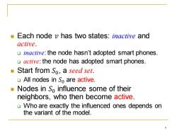
Each node v has two states:inactive and active. 0 inactive:the node hasn't adopted smart phones. 0 active:the node has adopted smart phones. Start from So,a seed set. All nodes in So are active. Nodes in So influence some of their neighbors,who then become active. Who are exactly the influenced ones depends on the variant of the model. 6

◼ Each node 𝑣 has two states: inactive and active. ❑ inactive: the node hasn’t adopted smart phones. ❑ active: the node has adopted smart phones. ◼ Start from 𝑆0, a seed set. ❑ All nodes in 𝑆0 are active. ◼ Nodes in 𝑆0 influence some of their neighbors, who then become active. ❑ Who are exactly the influenced ones depends on the variant of the model. 6

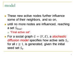
model These new active nodes further influence some of their neighbors,and so on, until no more nodes are influenced,reaching a set Sfinal. o“Final active set”. ■ For a social graph G=(V,E),a stochastic diffusion model specifies how active sets St, for all t≥1，is generated,given the initial seed set So

model ◼ These new active nodes further influence some of their neighbors, and so on, ◼ until no more nodes are influenced, reaching a set 𝑆final. ❑ “Final active set”. ◼ For a social graph 𝐺 = 𝑉, 𝐸 , a stochastic diffusion model specifies how active sets 𝑆𝑡 , for all 𝑡 ≥ 1, is generated, given the initial seed set 𝑆0. 7

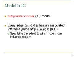
Model 1:IC Independent cascade (IC)model. Every edge (u,v)EE has an associated influence probability p(u,v)∈[0,1]· Specifying the extent to which node u can influence node v. 8

Model 1: IC ◼ Independent cascade (IC) model. ◼ Every edge 𝑢, 𝑣 ∈ 𝐸 has an associated influence probability 𝑝 𝑢, 𝑣 ∈ 0,1 • ❑ Specifying the extent to which node 𝑢 can influence node 𝑣. 8

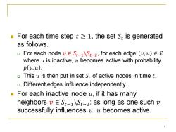
For each time step t =1,the set St is generated as follows. For each node vESt-1St-2,for each edge (v,u)EE where u is inactive,u becomes active with probability p(,u). This u is then put in set S;of active nodes in time t. Different edges influence independently. For each inactive node u,if it has many neighbors vE St-1St-2:as long as one such v successfully influences u,u becomes active. 9

◼ For each time step 𝑡 ≥ 1, the set 𝑆𝑡 is generated as follows. ❑ For each node 𝑣 ∈ 𝑆𝑡−1\𝑆𝑡−2 , for each edge 𝑣, 𝑢 ∈ 𝐸 where 𝑢 is inactive, 𝑢 becomes active with probability 𝑝 𝑣, 𝑢 . ❑ This 𝑢 is then put in set 𝑆𝑡 of active nodes in time 𝑡. ❑ Different edges influence independently. ◼ For each inactive node 𝑢, if it has many neighbors 𝑣 ∈ 𝑆𝑡−1\𝑆𝑡−2 : as long as one such 𝑣 successfully influences 𝑢, 𝑢 becomes active. 9

An equivalent model ■ Given a graph G=(V,E),we mark each edge (u,v)of G as either live or blocked. Pr[live]=p(u,v). The subgraph GL=(V,EL)where EL contains all the live edges. The step-t active set is R (So)={v:reachable from So within t steps} The final active set is defined as RGr (So)=RG(So)={v:reachable from So3 10

An equivalent model ◼ Given a graph 𝐺 = 𝑉, 𝐸 , we mark each edge 𝑢, 𝑣 of 𝐺 as either live or blocked. ❑ Pr 𝑙𝑖𝑣𝑒 = 𝑝 𝑢, 𝑣 . ◼ The subgraph 𝐺𝐿 = 𝑉, 𝐸𝐿 where 𝐸𝐿 contains all the live edges. ◼ The step-𝑡 active set is 𝑅𝐺𝐿 𝑡 𝑆0 = {𝑣: reachable from 𝑆0 within 𝑡 steps} ◼ The final active set is defined as 𝑅𝐺𝐿 𝑆0 = 𝑅𝐺𝐿 𝑛−1 𝑆0 = {𝑣: 𝑟𝑒𝑎𝑐ℎ𝑎𝑏𝑙𝑒 𝑓𝑟𝑜𝑚 𝑆0} 10